Difference between revisions of "Msc1G3:Grasshopper"

Latest revision as of 14:47, 19 December 2014

Grasshopper

Expert 3

@@ Line 20: / Line 20: @@
 </div><br>
-==Screenshots==
+==Screenshots Week 9==
+<gallery mode="packed-hover">
+Image: 14-12-19-step 1.jpg |
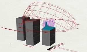
+Image: 14-12-19-step 2.jpg |Calculating the cut-outs for the existing floor slabs according to wind loads
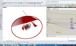
+Image: 14-12-19-step 3.jpg |Boundary surface for the new facade
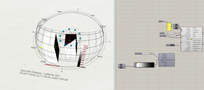
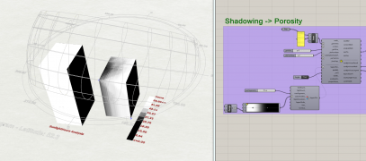
+Image: 14-12-19-step 4.jpg |Shadowing
+Image: 14-12-19-step 6.jpg |Assumed pathway through the landscape, projected to boundary surface
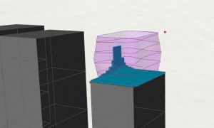
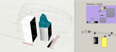
+Image: 14-12-19-step 7.jpg |Distribute the low "density" areas according to the shadow-diagram
+Image: 14-12-19-step 8.jpg |Distribute the high "density" areas according to the shadow-diagram
+Image: Step 9.PNG  |Map the low and dense areas to an array of 200 points
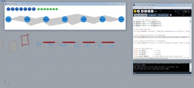
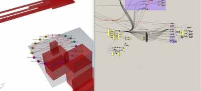
+Image: 14-12-19-step 12.jpg |Transfer Data to Processing - Watch Video
+Image: 14-12-19-step 13.jpg |Transfer Processingdata into Grasshopper
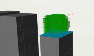
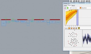
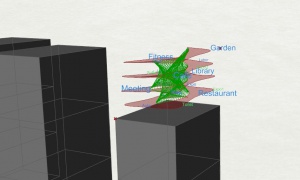
+Image: 14-12-19-step 14.jpg |Optimize the spatial distribution with galapagos
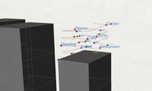
+Image: 14-12-19-step 15.jpg |Map the program to the pathway
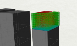
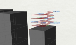
+Image: 14-12-19-step 16.jpg |Depth of the landscape dependent on the program
+Image: 14-12-19-step 17.jpg |Create wiring
+</gallery>
+==Videos Week 9==
+<html>
+<gallery>
+<iframe width="422" height="315" src="//www.youtube.com/embed/OBvYcNpQz1I" frameborder="0" allowfullscreen></iframe>
+</gallery>
+</html>
+==Screenshots Week 6==
 <gallery mode="packed-hover">
@@ Line 31: / Line 59: @@
 </gallery>
-==Videos==
+==Videos Week 6==
 <html>